School visited: Uncommon Collegiate Charter High School
Class observed: AP Grade 11 Statistics (UK equivalent Year 13)
Theme of post: Pedagogy and Curriculum
This is the second blog of a series to complement a workshop I delivered at #Mathsconf6 on Mathematics Pedagogy at USA Charter Schools, following my visiting a selection of Uncommon and North Star academy schools in New York and New Jersey. During the workshop, I discussed how the common denominator in each maths lesson I observed was the level of academic rigour. I am still trying to find a way to define this term, because it is overused and poorly defined.
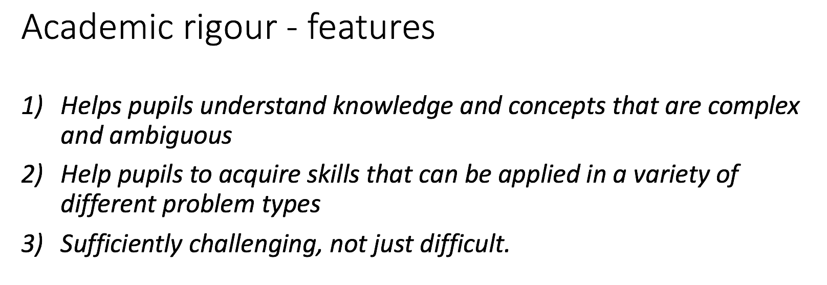
Nevertheless, I believe I can state that the teaching and learning delivered by such extraordinary teachers in the classrooms I observed displayed features of academic rigour. These features of academic rigour are evident in the structure of a teacher’s pedagogy and instruction:
In my workshop, I discussed the four main elements that all teachers up and down the country can implement into their teaching practice with minimal effort and maximum impact. I will discuss each of these four elements in turn, by way of one per blog post; today I will discuss the sequence of instruction.
I was observing a lesson, Grade 11 Statistics, and the teacher had organised the lesson so that he was trying to have pupils factorise cubic expressions where one of the expressions in the factorised form could be further factorised into two expressions because one group was a difference of two squares. (Figure 1) The sequence of instruction to explain to pupils how they can factorise such cubic expressions is what made his lesson so powerful.
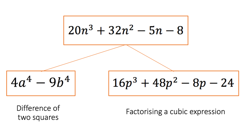 Figure 1 – Sequence of Instruction in terms of expressions used in teaching
Here, I entered the classroom, and the teacher had displayed the following algebraic expressions that he wanted pupils to factorise. (Figure 2) Before the pupils had even started to factorise he spent some time identifying the common features which determined this expression to be a difference of two squares. It is known as the difference of two squares because we have even powers, square numbers as coefficients and one positive term and one negative term.
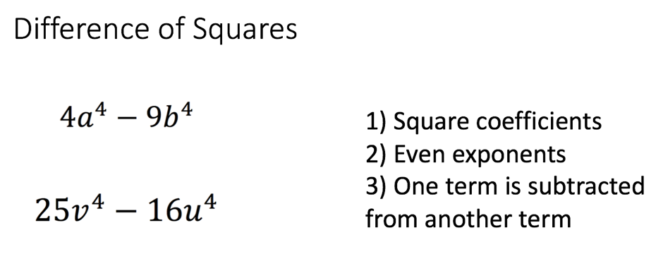 Figure 2 – Difference of two squares expressions + common features of this type of expression
What I found really fascinating was the examples that he had initially chosen in order to begin teaching pupils how to factorise such expressions. Previously, whilst teaching, I would begin teaching the topic by using the following examples and non-examples to state what the common features of an expression known as a difference of two squares actually looked like, and therefore what it would not look like. Therefore, I utilised simply examples and non-examples. (Figure 3)
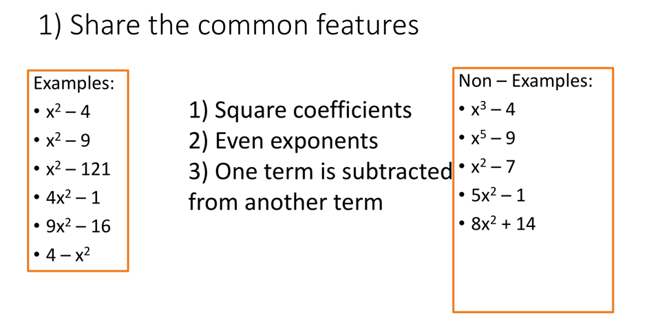
Figure 3 – Examples and Non examples used in the initial stages of teaching how to identify an expression known as a difference of two squares
The way the teacher started was better, because the expressions he had used made the common features more obvious to pupils. So the initial examples of a difference of two squares that I would have started to teach from are actually more nuanced and special; the coefficient of x2 being 1 is hidden, and instead of having two terms where the variables both have even powers we have a constant which is a square number.
Second, he then introduced the consistent algorithm he wanted pupils to use to go from the expanded form to the factorised form of the expression. He was very systematic (Figure 4 – consistent algorithm):
Step 1: square root both terms;
Step 2: divide both exponents by 2 and
Step 3: Write your answer as such.
He did this with a selection of examples, as you can see below:
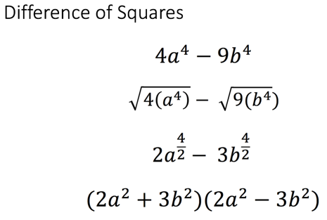
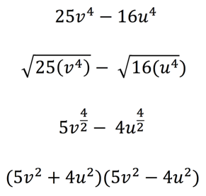
Figure 4 – Consistent algorithm to factorise an expression known as a difference of two squares
Following this, he then introduced the notion that the pupils would now learn how to factorise a cubic expression. At this point in the lesson, I wasn’t fully sure with where he was going (until we reached the end of the lesson). He stated that when we factorise a cubic expression as such we need to factorise the first two terms and the last two terms. He structured it for his pupils because he pre-empted a common mistake that pupils would have made unless he structured it for them. We are factorising the first two terms by dividing both terms by 1, whereas with the last two terms we are going to factorise by -1, because -1 is the greatest common factor of -8p and -24. (Figure 5) Therefore, the first step of the algorithm is not line 2: it is line 3. This was so powerful because by pre-empting this misconception, and by being very explicit with this instruction and guidance, it made the lesson run more smoothly because pupils were more independent to get on with the practice set of questions – because they weren’t making this mistake.
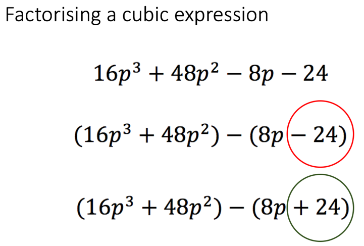
Figure 5 – Structuring the first step of the algorithm
He then carried on to lay out the consistent algorithm between the expanded form and the factorised form.
Step 1: factorise the first two terms, and the last two terms. (be careful when factorising the last two terms)
Step 2: Now factorise the greatest common factor for both terms (ensure that you are factorising the GCF of the coefficients as well as the variables) However, he posed the question one more time: “What is the greatest common factor of 16p^3 and 48p^2?” Students then noticed that we are no longer factorising by identifying the greatest common factor of the coefficients but also of the variables of each term. (Figure 6)
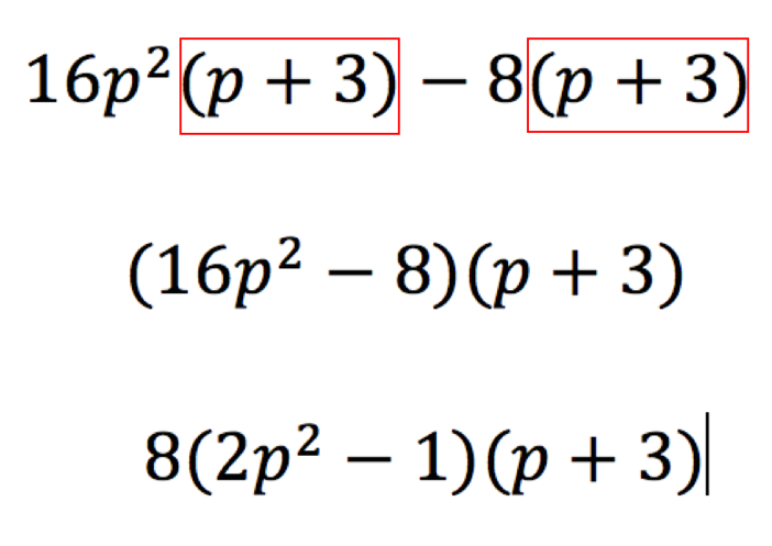
Figure 6 – Step 2 – Step 4 demonstrated
Step 3: factorise the greatest common binomial of the expression:
Again, the algorithm was consistent. Furthermore, he said factorise “the greatest common binomial”. This level of technical language being used in the classroom is fantastic, and is something I certainly intend to implement in my teaching practice.
Step 4: “Are we done with this problem?” he asked this question with the intent of having students identify that the first expression in parenthesis is not fully factorised – which pupils identified.
Here he paused and said to his pupils “Now you are thinking that we are finished because we have two groups that can then be expanded and simplified to form the expanded form which we start with, but we are not finished. What is the greatest common factor of the first group?” However, he posed the question one more time “What is the greatest common factor of 16p^2 and 8 ?”.Pupils then identified this to be 8. He then proceeded to do a selection of examples to complement the first example, and to also reiterate the consistent algorithm. Figure 7
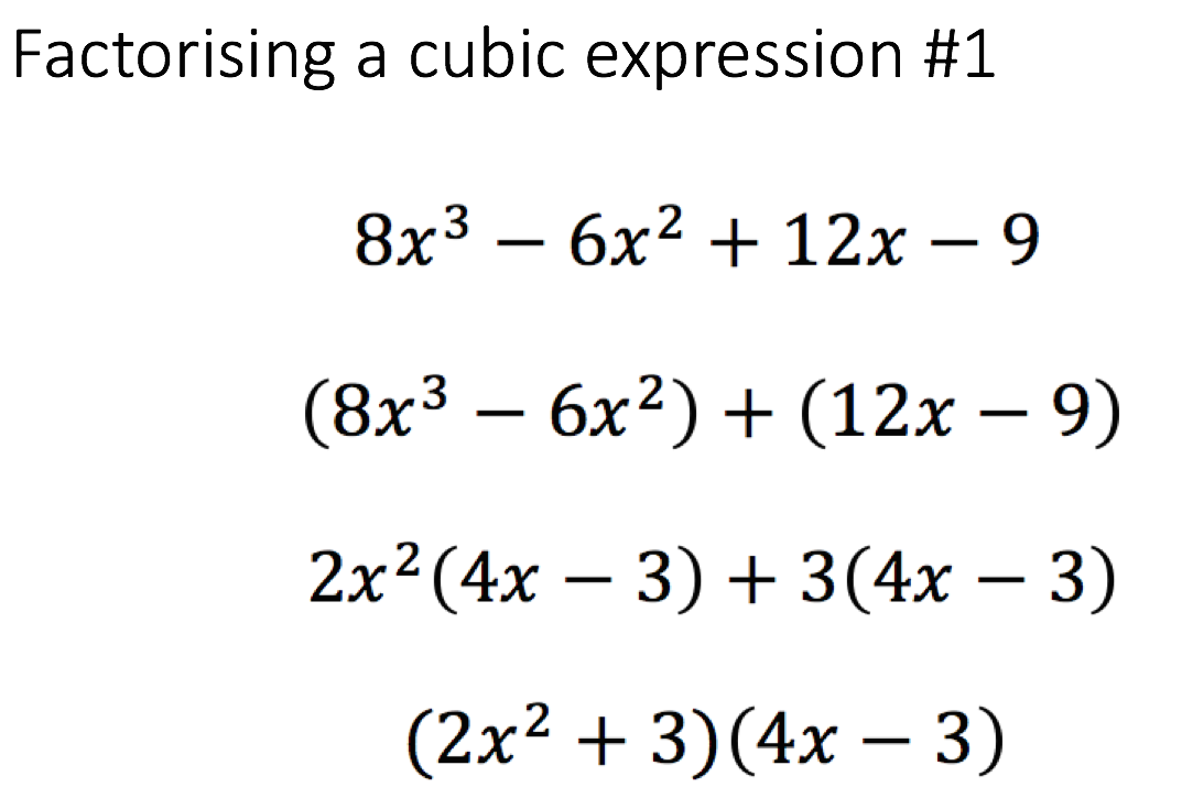
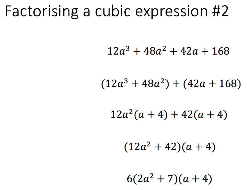
Figure 7 – Further examples of factorising cubic expressions presented in class using a consistent algorithm
Now, this was the pinnacle of the lesson. This was the point where the teacher introduced the next expression to factorise but in doing so he was combining the procedural knowledge of factorising a cubic expression where one of the groups could be factorised because it was a difference of two squares. The sequence of instruction was incredible. Let’s have a look.
Again, he used the consistent algorithm he showed in the previous examples:
Step 1: factorise the first two terms, and the last two terms. Pre-empt that we may be factorising the last two terms by 1 or -1.
Step 2: factorise the greatest common factor of both expressions:
Step 3: factorise the greatest common binomial of the expression.
He asked “can you factorise the greatest common factor of the second binomial? Hands up – what is the greatest common factor of the second binomial?” Pupils confidently answered – “1”. The teacher responded “Excellent, you can display it like this (teacher writes it on the board) and can you do the same on your mini-whiteboards please.” Again, he pre-empted another misconception that the pupils could have potentially made. (Figure 8)
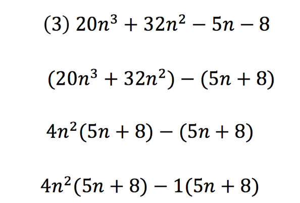
Figure 8 – Structuring a key step in the algorithm where pupils are more likely to make avoidable mistakes though explicit instruction.
Figure 9 – Introducing an expression where one group is an expression known as a difference of two squares
Step 4: factorise the greatest common binomial, which he got above (Figure 9):
He asked pupils to pause. He then asked pupils to look at the problem on the board (the one above). “Can you raise your hand when you can identify what type of binomial expression we have for the first binomial .” Ten hands were raised within the 5 seconds. In total there were 22 hands raised 10 seconds later. Now, after 30 seconds in total following the initial posing of the question, the teacher had an overall 28 out of 32 of pupils’ hands raised. The teacher selects a pupil to state the answer: “Sir, the first binomial is an expression which is a difference of two squares.”
The sequence of instruction here is incredibly effective. What I saw in real time, and what I have outlined for you, is not necessarily profound or extraordinary – on the contrary, it is very simple. It can be performed by all teachers.
It was evident from this lesson that the teacher had put a significant amount of thought into the sequence of his instruction to his pupils. It was well-crafted and sequenced so that all pupils could see the re-iterated key points. What are the characteristics of a problem which is a difference of two squares? What are the characteristics of factorising a non-linear expression? What is the greatest common factor of this expression – ensuring the greatest common factor including coefficients and variables?
I am still working on trying to collate a few different examples in my teaching practice of minimally different examples, and how I have interleaved concepts via sequence of instruction. I shall get back to you on this. Watch this space. Any questions then please do not hesitate to contact me or DM on twitter.
Leave a Reply
You must be logged in to post a comment.